
What are the odds that human civilization will be devastated, wiped out, or ‘reset’ by, say, a supervolcano? An asteroid impact? A pandemic? A.I. superintelligence deciding we’re obsolete? Nanoscale self-replicating machines consuming all biomass on Earth? The Large Hadron Collider creating a black hole that wipes out Earth?
For any such scenario, the stakes may range from regional devastation and global impact (supervolcano) to billions of deaths (pandemic), to, potentially, complete obliteration of humanity (black hole). High stakes to say the least.
Now, experts can try to estimate the probability of these high-stakes risks. For example, astronomers have cataloged most (not all) kilometer-sized near-Earth objects and determined from their orbital dynamics that none of the ones we’ve tracked will be a threat over the next 100 years; further models have attempted to estimate — with less certainty — the odds of those objects impacting over the next thousand years or longer (Fuentes-Munoz et al., 2023).
There are still, of course, smaller and more numerous near-Earth objects that could cause plenty of devastation (destroying cities or regions), plus the fact that we may have not have found all of the big ones to track.
Meanwhile, other ways of analyzing the risk may point to different conclusions. For example, reanalyzing large impact craters on Earth may end up adjusting our estimates of how often big objects have struck Earth in the past, which in turn is a decent way to estimate how often they’ll strike in the future on average. That alternate analysis rests partly on geological information and satellite imaging that are fuzzier than calculating the orbital dynamics of individual asteroids and comets we’re tracking, but may help us estimate the risk of smaller objects or converge on a similar estimate to the other risk models in a way that makes us more confident in those.
The larger point here, though, is that our estimation of any given low-probability risk can be imprecise. Some risks can be estimated with more confidence than others. Predicting pandemics is much harder than modeling where an asteroid you’re watching will end up 500 years from now. Predicting the odds of an AI-controlled robot uprising is even harder. I’m much more confident in the calculations of astronomers tracking individual objects in our solar system than I am in Ray Kurzweil predicting an AI-driven technological singularity by 2045, even though AI may end up being a greater threat. Some risks are just harder to predict than others.
However it is that we attempt to estimate and model these risks (which we should do, given the high stakes!), we have to accept some level of uncertainty in our models. This is the case with every model (for example, estimating whether there’s any effect of growth mindset interventions on school outcomes). Our scientific conclusions often come with some level of uncertainty, be it uncertainty in the magnitude or direction of an effect or even in the very existence of that effect. But when you are dealing with existential threats to humanity, that level of uncertainty becomes very, very important even for things that seem to have a low probability under some expert model.
A 2010 paper by Toby Ord and colleagues [PDF] says that we shouldn’t be quite so confident when we hear that the expert-assessed risk of some catastrophe is, say, one in a billion. Why? The chance that the expert’s methodology has some error or flaw in it may be higher than one in a billion, in which case the risk of that catastrophe may be significantly higher than we think.
Think of it this way: we want to know the probability of X occurring, where X is the catastrophe. Some researchers use their expertise and data to construct a scientific argument (call it A) that the risk is whatever it is, say one in a billion.
Ord and colleagues point out that what we really want to know is the probability of X, so we’ll call that P(X). But to get that we need to take into account the probability that argument A is correct and also the probability that it is wrong. We could denote those as P(A) and P(¬A), which you might verbalize in shorthand as “the probability of A” and “the probability of not A“.
Now, we know from probability theory that:
P(X) = P(X|A) P(A) + P(X|¬A) P(¬A)
…which may look overwhelming, but just bear with me; it’s not as crazy as it looks. Let me highlight two chunks of the equation here with some color and bold:
P(X) = P(X|A) P(A) + P(X|¬A) P(¬A)
What this is really saying is that the number we want — our best guess of the probability of catastrophe P(X) — comes from a combination of two things, which I’ve highlighted in blue and in red here.
First, the entire blue part thinks about “what if the scientist’s argument is correct”. The scientist has told us the probability of X, given A, usually written as P(X|A); they told us the odds of the catastrophe are one in a billion based on their argument. But we have to multiply that by the odds that their argument is correct! So we add P(A), the probability that A is correct. That’s what the blue chunk of the equation is calculating.
Just to throw a hypothetical number at it, imagine we assign their argument a 99% chance of being correct; then we’d be saying we think the probability of A is 0.99 (out of 1.0 being a certainty). In that case, the entire blue part in our hypothetical would be one in a billion (0.000000001) times 0.99, so the blue part of our equation would be 0.00000000099. (If you think the scientist’s argument has a 50% chance of being correct, you multiply one in a billion by 0.50, and if you think their argument has a 99.99% chance of being correct, you multiply by 0.9999, and so on).
So much for the blue side of the equation. We also have to account for the odds that their argument is wrong. That’s the red side of the equation, which, again, is:
P(X) = P(X|A) P(A) + P(X|¬A) P(¬A)
What is the probability of catastrophe X, given that the argument is mistaken? We’ll call that P(X|¬A), but unfortunately assigning a specific number to this is much harder (after all, if the best scientific estimate is wrong, then how would we know what the real risk is or what our guess of it should be?). Just realize that even if the argument A is wrong, there’s still some unknown chance of the catastrophe, maybe higher than their estimate, maybe lower).
Regardless, though, we have to multiply that by the odds that argument A is wrong. So if we previously said there was a 99% chance that A is correct (in the blue calculations), then we’d put 1% (a probability of 0.01) for P(¬A). If we thought the scientists’ argument had a 99.99% chance of being correct (a probability of 0.9999), then we’d say the probability of them being wrong is only a 0.0001. At any rate, we multiply this bit, P(¬A), by the P(X|¬A) to get the whole red part. The red part takes into account the what-if scenario when the scientist’s argument is wrong and also takes into account the chances of the scientist’s argument being wrong.
Why this big diversion into probability? To help you understand the figure below from Ord et al.’s (2010) paper. We’re used to thinking of catastrophic risks using the left box in the graph (the box presumably representing the whole space of what could happen). Scientists tell us the probability of some event happening, P(X), and that’s the black bar at the bottom of the box; the rest of the probability space is the white area. If the black bar is super, super thin (say, one in a billion), it’s easy to mistakenly think about the probability in this simplified way (the left-hand box). But what we really should be thinking about is the right-hand box, which I’ll explain below.
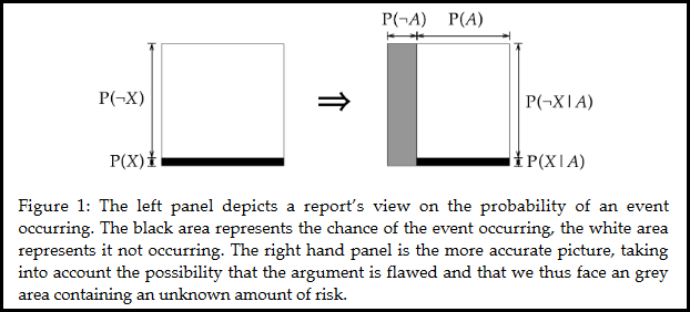
The right-hand box just copies the original box (the black portion and white portion), but adds a new chunk to the probability space (the gray portion). Notice how the black and white parts are all located under P(A); the black and white parts are when we assume that the argument is correct. But we have to also consider the gray possibility (the odds that the argument is wrong), within which is some sub-area representing the probability of catastrophe X then.
We don’t know exactly how big the gray area is because we can’t be precisely sure how confident to be in the scientist’s argument. But if the black bar is super tiny (say, one in a billion is the scientist’s estimate) then even a small chance of the scientist being wrong (say, one in ten thousand) could dwarf the black space with a big gray area of uncertainty.
Now, the gray area is not the actual odds of our catastrophe happening when the scientist is wrong. It’s not showing us P(X|¬A) even though that is what we really want (we really want to know the sub-part of the gray area that represents our risk even when the scientist’s argument is wrong; combine that with black and we know the actual risk!).
Conceptually, though, even though we don’t know exactly how big the gray section is or what the sub-part of the gray section would be (for risk when the scientist is wrong), we can use this figure to see how the scientist’s risk estimate (the black section) is utterly incomplete.
Maybe the gray bar is small (1% of the total box), but if the black bar is incredibly tiny (0.0000001%, one in a billion), then the unknown sub-part of the gray bar that we’re worried about may still be bigger than the black bar itself. Perhaps much bigger. In which case, the risk of X would be the combination of the black bar and this unknown but much bigger area. The risk in that case is much worse than it initially seemed given the scientist’s modeling of a one in a billion chance.
Ord’s paper goes on to argue that scientific arguments end up being wrong more than we might like (for various reasons like errors in theory, in models borne out of those theories, or even in calculations), so P(¬A) isn’t something we can ignore. The gray box may be bigger than we usually think!
Of course, we’ve been talking in rather binary terms about the scientist’s argument (their estimate) being correct or incorrect. In reality, any estimate (like the hypothetical one in a billion) comes with uncertainty, with a baked-in margin of error. Any scientist who understands what they’re doing will not be telling us “the metaphysical chances of this event occurring are exactly 0.000000001”; they’re giving us something akin to a point estimate, a single number representing a sort of middle point in a distribution of possibilities based on the probabilistic model they created. Scientists know that their models have uncertainty. Indeed, the exact number given by the point estimate is basically guaranteed to be wrong, but hopefully only a little bit wrong (the probabilistic model can tell us how likely it is to be wrong by a given amount, but that in turn relies on the assumptions of the model).
The point is: a researcher estimating the risk of something is presenting us with a single number as a sort of representative glimpse at a fuzzy, uncertain projection. What Ord and colleagues (2010) are really adding on here, I think, is that the method used to construct that fuzzy, uncertain projection is itself based on additional layers of uncertainty (the assumptions that go into the scientist’s probabilistic model may also be in error, not just in a binary way, but in magnitude or direction of effect, say).

It’s hard, damn hard, for us humans to think in terms of uncertainties, especially when those uncertainties are layered on each other. But it’s important, because when it comes to something with stakes as high as billions of deaths or even the end of humanity, fuzziness and uncertainty about low probability events can make a big difference. It’s not necessarily the case every time, but at least sometimes, the odds may be significantly worse than our best models tell us. And even though this may represent a small increase in absolute odds for our low-probability events (they’ll still be low probability!), an additional, say, one in a million chance of humanity disappearing is something to pay attention to.
That’s not to say that this is cause for panic or pessimism; it just means that when we do the serious job of estimating the odds of low-probability, high-stakes events, we need to consider that our estimates rely on theories, models, and calculations which themselves involve uncertainties, and we need to keep in mind that this means the real risk of some of those events may be higher than our best estimates project.
Why does this matter, if the absolute probability is still quite low? I’ll leave that for another post, but if you want to read more, Nick Bostrom, for example, has written about existential risk prevention and how to metaphorically (or literally) put a number to the loss in the case of an unlikely catastrophic outcome (see Bostrom, 2013 for a representative publication).
*****
On a related note:
Thinking about things with very low probability but very high stakes reminds me a bit of Pascal’s Wager. As an argument for believing in a particular god — like all the versions of the Christian god on offer — it’s all-around pretty weaksauce (though Pascal wasn’t explicitly using it as a rational argument for his god’s existence). That said, the popularized, rhetorical version of Pascal’s Wager deals with things like “infinite loss” as a possible outcome, something which sounds similar to “end of humanity” outcomes in the existential risk calculations above.
One might assign a very small subjective probability to the chance of a particular humanity-ending event occurring (e.g., Large Hadron Collider spawns a black hole that wipes out the Earth) similar to how some might assign a very small subjective probability to the chance that there exists a particular version of a particular god (the versions found in different branches and sects of Islam, Christianity, Mormonism, etc.); but the stakes of these low probability events are quite high.
That’s the surface similarity to Pascal’s Wager, anyway. There are various reasons I don’t find the wager at all convincing, so it may be interesting to interrogate why one might be much more convinced by arguments that we should act now to avoid existential risks to humanity (when we find the probability of those risks very low).
*****
References
Bostrom, N. (2013). Existential risk prevention as global priority. Global Policy, 4(1), 15-31. https://doi.org/10.1111/1758-5899.12002 [PDF]
Fuentes-Munoz, O., Scheeres, D. J., Farnocchia, D., & Park, R. S. (2023). The hazardous km-sized NEOs of the next thousands of years. The Astronomical Journal. https://doi.org/10.48550/arXiv.2305.04896 [PDF]
Ord, T., Hillerbrand, R., & Sandberg, A. (2010). Probing the improbable: Methodological challenges for risks with low probabilities and high stakes. Journal of Risk Research, 13(2), 191-205. DOI: https://doi.org/10.1080/13669870903126267 [SciHub PDF]
Leave a Reply